#Note: lines are commented with a # sign. If not they don't have a # in the beginning it means they are the commands of the R code.
# STEP 1. Installing packages and fixing the data sets:
# We should first install some packages:
install.packages("akima")
install.packages("EcoHydRology")
install.packages("hydroGOF")
install.packages("rootSolve")
#Later we should call the packages into the environment
library(EcoHydRology)
library(hydroTSM)
library(akima)
library(lubridate)
library(hydroGOF)
library(rootSolve)
library(ggplot2)
library(directlabels)
#STEP 2. Declare the functions.
#2.1 Calculate values based on the WV Water year (Function Written by Dr. Nicolas Zegre)
FernowWaterYear <-function (x)
{
yr <- year(x)
ifelse(month(x, label = FALSE) > 4, yr+1, yr)
}
#2.2 This functions is used to generate n value based on Budyko Equation (1) in Roderick and Farquhar 2011.
calibn<-function(n,p,ep,e)
{
(p*ep)/((p^n+ep^n)^(1/n))-e
}
#STEP 3. Get and fix the data needed for the Analysis (P, Q, PET).
#3.1 Obtain Potential Evapotranspiration: Begins PET-Priestly Taylor Analysis:
ftempi<-read.csv(file="~/Google Drive/Ref_catchments/Data/ftemp_interp_wjulian_day.csv", header=TRUE, sep = ",")
tdpet=seq(as.Date("1951/8/1"), as.Date("2013/12/31"), by="day")
attach(ftempi)
# LATITUDE TO RADIANS, WS1 weir coordinate: 39.05387N 79.68258W
lat<-39.05387
rad<-(lat*pi)/180
ws4pet_pt<-PET_fromTemp(JULIANDAY,TMAX,TMIN,rad,AvgT=TAVG, albedo = 0.15, TerrestEmiss = 0.97,forest = 0, PTconstant = 1.26 )
detach(ftempi)
# PET Annual Analysis #
tdpet=seq(as.Date("1951/8/1"), as.Date("2012/12/31"), by="day")
pet<-1000*(ws4pet_pt)
pet.z<-zoo(x=pet, order.by=tdpet)
#Apply Water year function:
ewyr<-FernowWaterYear(pet.z)
WATERYEARpet<-ewyr-1
#aggregate to annual values
pet.wyr<-tapply(pet.z,WATERYEARpet, FUN=sum, na.rm=TRUE)
#Spline to correct in case of missing values
pet.wyr2<-pet.wyr
pet.wyr[57]<-NA
pet.zna<-na.spline(pet.wyr)# Spline Interpolate for year 2007
pet.wyr2[57]<-1021.3810 #1021.3810 was the result the spline function put in year 2007
pet.ss<-pet.wyr2[2:61]
#3.2.Obtain Q:
fr<-read.csv(file="Data/q_fernow.csv", sep=",", header=TRUE)
td=seq(as.Date("1952/01/01"), as.Date("2013/12/31"), "days")
qdaily<-(fr$ws4)
qdaily.z<-zoo(x=qdaily, order.by=td)
# determine water year
qwyr<-FernowWaterYear(qdaily.z)
# Trims dataset to exclude incomplete shoulder years
WATERYEARq <- qwyr-1
#aggregates to annual runoff
aqt<-tapply(qdaily.z,WATERYEARq, FUN=sum, na.rm=TRUE)
aq<-aqt[2:61] #trims water years to only from 1952 to 2011
#3.3 Obtain P
P<-read.csv(file="Data/p_fernow.csv", sep=",", header=TRUE)
tdp=seq(as.Date("1951/05/01"), as.Date("2013/12/31"), "days")
dailyp<-(P$p_ws4)
p.z<-zoo(x=dailyp, order.by=tdp)
pwyr<-FernowWaterYear(p.z)
WATERYEARp<-pwyr-1
apt<-tapply(p.z,WATERYEARp, FUN=sum, na.rm=TRUE)
ap<-apt[2:61]
# Step 4. Calculate the Evaporative Index and Dryness Index
#Annual Actual evapotranspiration: P-Q
aet<-ap-aq
# Evaporative index = P-Q/P
ei<-aet/ap
# Dryness index = pet/p
dry<-pet.ss/ap
str(ei)
str(dry)
range(ei) # 0.2545175 0.7583817
range(dry) #0.5663119 0.9941203
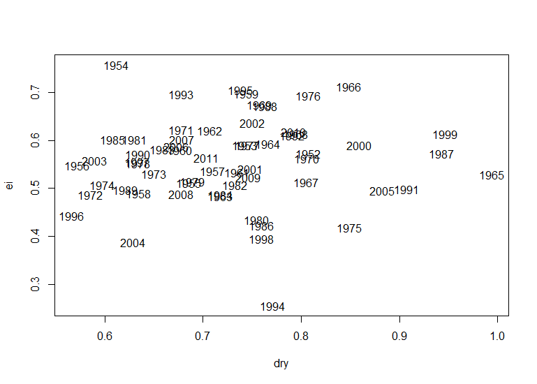
plot(dry,ei, type="n")
text(dry,ei, label=c(1952:2011))
#Lets see the resulting plot of the all the years Dryness Index vs Evaporative Index:
# STEP 1. Installing packages and fixing the data sets:
# We should first install some packages:
install.packages("akima")
install.packages("EcoHydRology")
install.packages("hydroGOF")
install.packages("rootSolve")
#Later we should call the packages into the environment
library(EcoHydRology)
library(hydroTSM)
library(akima)
library(lubridate)
library(hydroGOF)
library(rootSolve)
library(ggplot2)
library(directlabels)
#STEP 2. Declare the functions.
#2.1 Calculate values based on the WV Water year (Function Written by Dr. Nicolas Zegre)
FernowWaterYear <-function (x)
{
yr <- year(x)
ifelse(month(x, label = FALSE) > 4, yr+1, yr)
}
#2.2 This functions is used to generate n value based on Budyko Equation (1) in Roderick and Farquhar 2011.
calibn<-function(n,p,ep,e)
{
(p*ep)/((p^n+ep^n)^(1/n))-e
}
#STEP 3. Get and fix the data needed for the Analysis (P, Q, PET).
#3.1 Obtain Potential Evapotranspiration: Begins PET-Priestly Taylor Analysis:
ftempi<-read.csv(file="~/Google Drive/Ref_catchments/Data/ftemp_interp_wjulian_day.csv", header=TRUE, sep = ",")
tdpet=seq(as.Date("1951/8/1"), as.Date("2013/12/31"), by="day")
attach(ftempi)
# LATITUDE TO RADIANS, WS1 weir coordinate: 39.05387N 79.68258W
lat<-39.05387
rad<-(lat*pi)/180
ws4pet_pt<-PET_fromTemp(JULIANDAY,TMAX,TMIN,rad,AvgT=TAVG, albedo = 0.15, TerrestEmiss = 0.97,forest = 0, PTconstant = 1.26 )
detach(ftempi)
# PET Annual Analysis #
tdpet=seq(as.Date("1951/8/1"), as.Date("2012/12/31"), by="day")
pet<-1000*(ws4pet_pt)
pet.z<-zoo(x=pet, order.by=tdpet)
#Apply Water year function:
ewyr<-FernowWaterYear(pet.z)
WATERYEARpet<-ewyr-1
#aggregate to annual values
pet.wyr<-tapply(pet.z,WATERYEARpet, FUN=sum, na.rm=TRUE)
#Spline to correct in case of missing values
pet.wyr2<-pet.wyr
pet.wyr[57]<-NA
pet.zna<-na.spline(pet.wyr)# Spline Interpolate for year 2007
pet.wyr2[57]<-1021.3810 #1021.3810 was the result the spline function put in year 2007
pet.ss<-pet.wyr2[2:61]
#3.2.Obtain Q:
fr<-read.csv(file="Data/q_fernow.csv", sep=",", header=TRUE)
td=seq(as.Date("1952/01/01"), as.Date("2013/12/31"), "days")
qdaily<-(fr$ws4)
qdaily.z<-zoo(x=qdaily, order.by=td)
# determine water year
qwyr<-FernowWaterYear(qdaily.z)
# Trims dataset to exclude incomplete shoulder years
WATERYEARq <- qwyr-1
#aggregates to annual runoff
aqt<-tapply(qdaily.z,WATERYEARq, FUN=sum, na.rm=TRUE)
aq<-aqt[2:61] #trims water years to only from 1952 to 2011
#3.3 Obtain P
P<-read.csv(file="Data/p_fernow.csv", sep=",", header=TRUE)
tdp=seq(as.Date("1951/05/01"), as.Date("2013/12/31"), "days")
dailyp<-(P$p_ws4)
p.z<-zoo(x=dailyp, order.by=tdp)
pwyr<-FernowWaterYear(p.z)
WATERYEARp<-pwyr-1
apt<-tapply(p.z,WATERYEARp, FUN=sum, na.rm=TRUE)
ap<-apt[2:61]
# Step 4. Calculate the Evaporative Index and Dryness Index
#Annual Actual evapotranspiration: P-Q
aet<-ap-aq
# Evaporative index = P-Q/P
ei<-aet/ap
# Dryness index = pet/p
dry<-pet.ss/ap
str(ei)
str(dry)
range(ei) # 0.2545175 0.7583817
range(dry) #0.5663119 0.9941203
plot(dry,ei, type="n")
text(dry,ei, label=c(1952:2011))
#Lets see the resulting plot of the all the years Dryness Index vs Evaporative Index:
#Step 5. Budyko decomposition.
#Calculate means for the whole period of record
ap1<-mean(ap)
aq1<-mean(aq)
aet1<-mean(aet)
pet1<-mean(pet.ss)
ei1<-mean(ei)
dry1<-mean(dry)
#Aggregate via a bi-period time step
byperiod <- rep(1:2, each = 30)
ei2<-zoo(aggregate(ei, list(byperiod),mean)) #evap index divided in two periods
dry2<-zoo(aggregate(dry, list(byperiod),mean)) #dryness index divided in two 30 years periods
ap2<-zoo(aggregate(ap, list(byperiod),mean)) #precipitation divided in two 30 yr periods
pet2<-zoo(aggregate(pet.ss,list(byperiod),mean))#potential evapotranspiration divided in two 30 yr periods
aq2<-zoo(aggregate(aq, list(byperiod),mean)) #total annual runoff
aet2<-zoo(aggregate(aet, list(byperiod),mean)) #total annual evaporation
write.csv(cbind(range(ei),range(dry),ei2,dry2,ap2,aq2,pet2,aet2), file="period_B_D_variable.csv" )
#Calculate n, applying the function we declared at the beginning and using the package rootSolve to calibrate n
n_value<-uniroot.all(calibn,c(.01,1000),tol=.000001,p=mean(ap),ep=mean(pet.ss),e=mean(aet))
n<-n_value[1]
#Use Budyko Equation to calculate AET
AET.1<-(ap*pet.ss)/((ap^n+pet.ss^n)^(1/n))
aet_c<-(ap1*pet1)/((ap1^n+pet1^n)^(1/n))
#Calculate the Sensitivity coeficients (equations 5a,b,c from Roderick and Farquhar, 2011)
dE_dP<-(aet1/ap1)*(pet1^n)/(ap1^n+pet1^n) #Eq 5a
dE_dPET<-(aet1/pet1)*(ap1^n)/(ap1^n+pet1^n) #Eq 5b
dE_dn<-(aet1/n)*(log(ap1^n+pet1^n)/n-(((ap1^n)*log(ap1)+(pet1^n)*log(pet1))/(ap1^n+pet1^n))) #Eq 5c
#Calculate the differences between the historical and second period
dn<-0 # Considering that the landscape has not changed. n=0
dP<-as.numeric(ap2[2,2])-as.numeric(ap1) # Difference in P between the periods
dPET<-as.numeric(pet2[2,2])-as.numeric(pet1) # Difference in PET between periods
dAET<- dE_dP*dP+dE_dPET*dPET+dE_dn*dn #Eq 4. using the values found using Eq 5
dQ<-dP-dAET #Eq 6 OBS: Equations 4 and 6 should give the same value!!)
dQ1<-(1-dE_dP)*dP-dE_dPET*dPET-dE_dn*dn # Associated change in Q. Eq 7
dQ_Q<-(ap1/aq1*(1-dE_dP))*(dP/ap1)-(pet1/aq1)*dE_dPET*(dPET/pet1)-(n/aq1)*dE_dn*(dn/n) #relative change in Q Eq. 8
dQ_dP<-1-dE_dP
#Calculate the Sensitivity Coefficients of equation 8 in Roderick and Farquhar, 2011.
scP<-(ap1/aq1*(1-dE_dP))
scPET<-(pet1/aq1)*dE_dPET
scn<-(n/aq1)*dE_dn
#Sensitivity results output
result<-cbind(dn,dP,dPET,dAET,dQ,dQ1,dQ_Q,dQ_dP,dE_dP,dE_dPET,dE_dn,n,scP,scPET,scn)
#STEP 6. Ploting some of the results:
# Plot the Budyko Curve
x=seq(0,2,by=.0333)
x<-x[1:60]
n<-1.74
y1<- x/((1+x^n)^(1/n)) #ecuation of Evaporative Index from Choudhury 1999.
y2<-x/((1+x^1.8)^(1/1.8))
bc<-data.frame(dry,ei,aq,ap,pet.ss,aet,AET.1,pet.ss-aet)
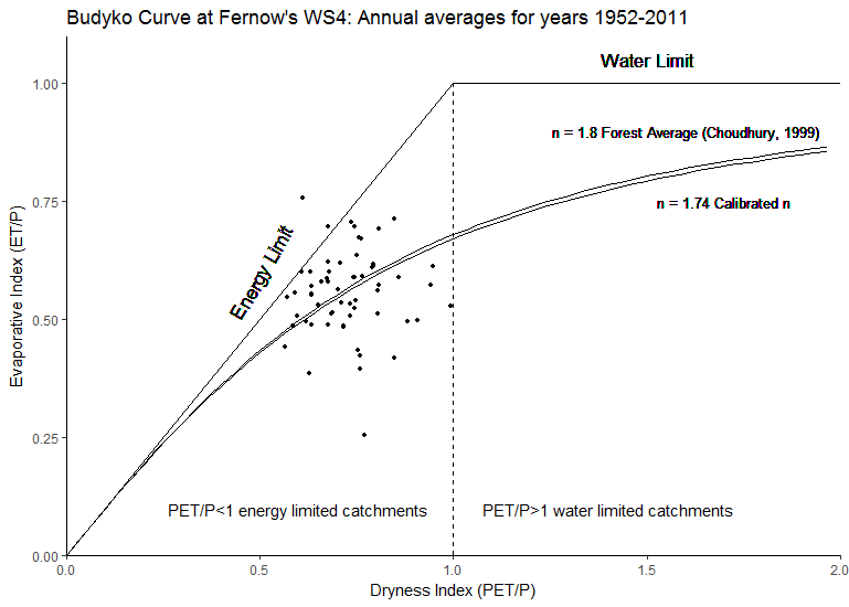
a<-ggplot(data=bc)+aes(dry,ei)+theme_classic()+scale_x_continuous(expand = c(0,0),limits = c(0,2))+
ggtitle("Budyko Curve at Fernow's WS4: Annual averages for years 1952-2011")+
scale_y_continuous(expand = c(0, 0),limits=c(0,1.1))+scale_shape_discrete(solid=F)+
annotate("text", x = 0.6, y = 0.1, label = "PET/P<1 energy limited catchments")+
annotate("text",x=1.4,y=0.1,label="PET/P>1 water limited catchments")+
geom_point(aes(x=dry,y=ei),size=1,show.legend = FALSE)+
geom_text(x=1.6,y=0.9,aes(label="n = 1.8 Forest Average (Choudhury, 1999)"), size=3.5)+
geom_text(x=1.7,y=0.75,aes(label="n = 1.74 Calibrated n"), size=3.5)
b<-labs(x="Dryness Index (PET/P)",y="Evaporative Index (ET/P)",size=2)
c<-geom_segment(aes(x = 0, y = 0, xend = 1, yend = 1))
d<-geom_segment(aes(x=1,y=1,xend=2,yend=1))
e<-geom_segment(aes(x=1,y=0,xend=1,yend=1),linetype=2)
f<-geom_text(x=0.5,y=0.6,aes(label="Energy Limit",angle=60, size=1.5),show.legend = FALSE) #Water limit label
g<-geom_text(x=1.5,y=1.05,aes(label="Water Limit",size=1.5),show.legend = FALSE) #Energy Limit label
h<-geom_line(aes(x=x,y=y1))
i<-geom_line(aes(x=x,y=y2))
budyko<-a+b+c+d+e+f+g+h+i
budyko
#Calculate means for the whole period of record
ap1<-mean(ap)
aq1<-mean(aq)
aet1<-mean(aet)
pet1<-mean(pet.ss)
ei1<-mean(ei)
dry1<-mean(dry)
#Aggregate via a bi-period time step
byperiod <- rep(1:2, each = 30)
ei2<-zoo(aggregate(ei, list(byperiod),mean)) #evap index divided in two periods
dry2<-zoo(aggregate(dry, list(byperiod),mean)) #dryness index divided in two 30 years periods
ap2<-zoo(aggregate(ap, list(byperiod),mean)) #precipitation divided in two 30 yr periods
pet2<-zoo(aggregate(pet.ss,list(byperiod),mean))#potential evapotranspiration divided in two 30 yr periods
aq2<-zoo(aggregate(aq, list(byperiod),mean)) #total annual runoff
aet2<-zoo(aggregate(aet, list(byperiod),mean)) #total annual evaporation
write.csv(cbind(range(ei),range(dry),ei2,dry2,ap2,aq2,pet2,aet2), file="period_B_D_variable.csv" )
#Calculate n, applying the function we declared at the beginning and using the package rootSolve to calibrate n
n_value<-uniroot.all(calibn,c(.01,1000),tol=.000001,p=mean(ap),ep=mean(pet.ss),e=mean(aet))
n<-n_value[1]
#Use Budyko Equation to calculate AET
AET.1<-(ap*pet.ss)/((ap^n+pet.ss^n)^(1/n))
aet_c<-(ap1*pet1)/((ap1^n+pet1^n)^(1/n))
#Calculate the Sensitivity coeficients (equations 5a,b,c from Roderick and Farquhar, 2011)
dE_dP<-(aet1/ap1)*(pet1^n)/(ap1^n+pet1^n) #Eq 5a
dE_dPET<-(aet1/pet1)*(ap1^n)/(ap1^n+pet1^n) #Eq 5b
dE_dn<-(aet1/n)*(log(ap1^n+pet1^n)/n-(((ap1^n)*log(ap1)+(pet1^n)*log(pet1))/(ap1^n+pet1^n))) #Eq 5c
#Calculate the differences between the historical and second period
dn<-0 # Considering that the landscape has not changed. n=0
dP<-as.numeric(ap2[2,2])-as.numeric(ap1) # Difference in P between the periods
dPET<-as.numeric(pet2[2,2])-as.numeric(pet1) # Difference in PET between periods
dAET<- dE_dP*dP+dE_dPET*dPET+dE_dn*dn #Eq 4. using the values found using Eq 5
dQ<-dP-dAET #Eq 6 OBS: Equations 4 and 6 should give the same value!!)
dQ1<-(1-dE_dP)*dP-dE_dPET*dPET-dE_dn*dn # Associated change in Q. Eq 7
dQ_Q<-(ap1/aq1*(1-dE_dP))*(dP/ap1)-(pet1/aq1)*dE_dPET*(dPET/pet1)-(n/aq1)*dE_dn*(dn/n) #relative change in Q Eq. 8
dQ_dP<-1-dE_dP
#Calculate the Sensitivity Coefficients of equation 8 in Roderick and Farquhar, 2011.
scP<-(ap1/aq1*(1-dE_dP))
scPET<-(pet1/aq1)*dE_dPET
scn<-(n/aq1)*dE_dn
#Sensitivity results output
result<-cbind(dn,dP,dPET,dAET,dQ,dQ1,dQ_Q,dQ_dP,dE_dP,dE_dPET,dE_dn,n,scP,scPET,scn)
#STEP 6. Ploting some of the results:
# Plot the Budyko Curve
x=seq(0,2,by=.0333)
x<-x[1:60]
n<-1.74
y1<- x/((1+x^n)^(1/n)) #ecuation of Evaporative Index from Choudhury 1999.
y2<-x/((1+x^1.8)^(1/1.8))
bc<-data.frame(dry,ei,aq,ap,pet.ss,aet,AET.1,pet.ss-aet)
a<-ggplot(data=bc)+aes(dry,ei)+theme_classic()+scale_x_continuous(expand = c(0,0),limits = c(0,2))+
ggtitle("Budyko Curve at Fernow's WS4: Annual averages for years 1952-2011")+
scale_y_continuous(expand = c(0, 0),limits=c(0,1.1))+scale_shape_discrete(solid=F)+
annotate("text", x = 0.6, y = 0.1, label = "PET/P<1 energy limited catchments")+
annotate("text",x=1.4,y=0.1,label="PET/P>1 water limited catchments")+
geom_point(aes(x=dry,y=ei),size=1,show.legend = FALSE)+
geom_text(x=1.6,y=0.9,aes(label="n = 1.8 Forest Average (Choudhury, 1999)"), size=3.5)+
geom_text(x=1.7,y=0.75,aes(label="n = 1.74 Calibrated n"), size=3.5)
b<-labs(x="Dryness Index (PET/P)",y="Evaporative Index (ET/P)",size=2)
c<-geom_segment(aes(x = 0, y = 0, xend = 1, yend = 1))
d<-geom_segment(aes(x=1,y=1,xend=2,yend=1))
e<-geom_segment(aes(x=1,y=0,xend=1,yend=1),linetype=2)
f<-geom_text(x=0.5,y=0.6,aes(label="Energy Limit",angle=60, size=1.5),show.legend = FALSE) #Water limit label
g<-geom_text(x=1.5,y=1.05,aes(label="Water Limit",size=1.5),show.legend = FALSE) #Energy Limit label
h<-geom_line(aes(x=x,y=y1))
i<-geom_line(aes(x=x,y=y2))
budyko<-a+b+c+d+e+f+g+h+i
budyko
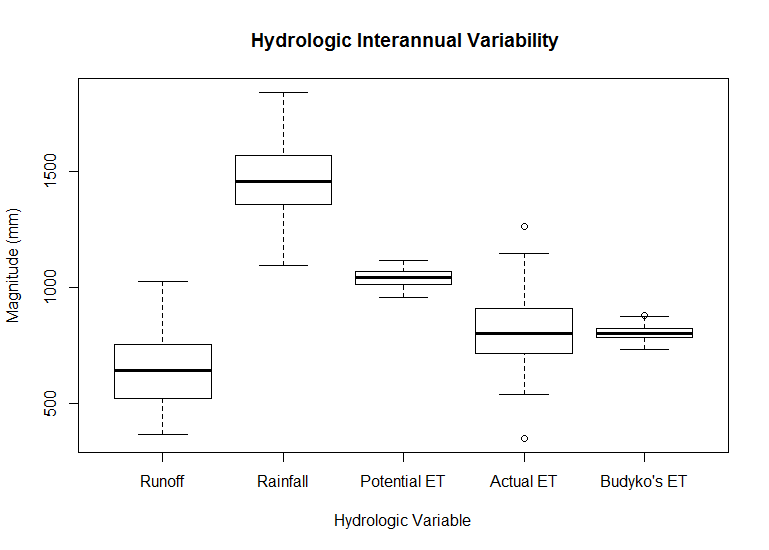
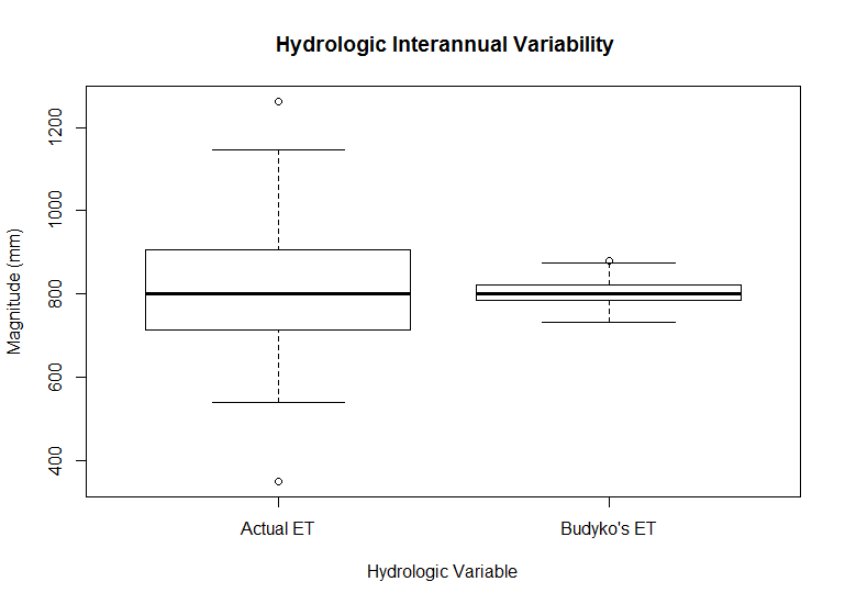
#Plot Blox plots to see some of the variability in the Hydrological variables.
boxplot(bc[,3:7],main=" Hydrologic Interannual Variability", ylab="Magnitude (mm)", xlab="Hydrologic Variable",names=c("Runoff","Rainfall","Potential ET","Actual ET","Budyko's ET") )
boxplot(bc[,6:7],main=" Hydrologic Interannual Variability", ylab="Magnitude (mm)", xlab="Hydrologic Variable",names=c("Actual ET","Budyko's ET") )
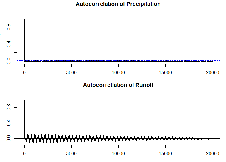
#Plot Autocorrelations of Precipitation and Runoff.
par(mfrow=c(2,1), mar=c(3,3,3,1))
acf(dailyp, lag.max=20000,ylab="ACF(daily P)",main="Autocorrelation of Precipitation")
acf(qdaily,lag.max=20000, ylab="ACF(Daily Q)",main="Autocorretlation of Runoff")
par(new=F)
dev.off()
par(mfrow=c(2,1), mar=c(3,3,3,1))
acf(dailyp, lag.max=20000,ylab="ACF(daily P)",main="Autocorrelation of Precipitation")
acf(qdaily,lag.max=20000, ylab="ACF(Daily Q)",main="Autocorretlation of Runoff")
par(new=F)
dev.off()
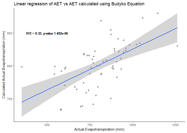
#Plot Linear Regression of the AET and AETc (calculated using the Budyko Framework)
fitplot<-ggplot(bc, aes(x=aet, y=AET.1))+theme_classic() + #"aesthetic mappings"
geom_point(shape=1) + # Use hollow circles
geom_smooth(method=lm)+ # Add linear regression line (by default includes 95% confidence region)
geom_text(x=500,y=850,aes(label="R^2 = 0.32, p-value 1.402e-06"), size=3.5)+
labs(x="Actual Evapotranspiration (mm)",y="Calculated Actual Evapotranspiration (mm)",size=2)+
ggtitle("Linear regression of AET vs AET calculated using Budyko Equation")
fitplot
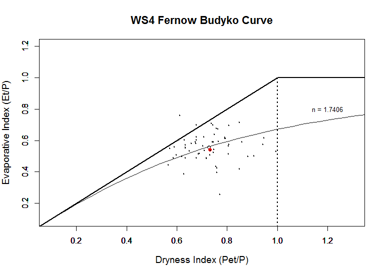
#Other form of Plotting the Budyko Curve using the more simpler plot function: (This code was originially written by Dr. Nicolas Zegre).
lin1x<-c(0.0,1)
lin1y<-c(0.0,1)
lin2x<-c(1,2)
lin2y<-c(1,1)
lin3x<-c(1,1)
lin3y<-c(0.0,1.0)
plot(lin1x, lin1y, type="l",lwd="2", xlim=c(0.1,1.3), ylim=c(0.1, 1.2),
ylab="", xlab="", col= "black", main="")
par(new=T)
plot(lin2x, lin2y, type="l", lwd="2",xlim=c(0.1,1.3), ylim=c(0.1, 1.2),
xlab="", ylab="", col="black")
par(new=T)
plot(lin3x, lin3y, type="l",lty=3, lwd="2",xlim=c(0.1,1.3), ylim=c(.1, 1.2),
xlab="", ylab="", col="black")
par(new=T)
plot(x, y1, type="l", xlim=c(.1,1.3), ylim=c(.1, 1.2), lty=1, cex.lab=1.2,cex.main=1.4, ylab="Evaporative Index (Et/P)", xlab="Dryness Index (Pet/P)", col= "gray5", main="WS4 Fernow Budyko Curve")
text(1.2,0.8,label="n = 1.7406",cex=0.8)
par(new=T)
plot(dry1,ei1, type="p",xlim=c(.1,1.3), ylim=c(.1, 1.2), ylab="", xlab="", main=" ",col="BLACK",pch=1)
par(new=T)
plot(dry2[2,2],ei2[2,2], type="p",xlim=c(.1,1.3), ylim=c(.1, 1.2), ylab="", xlab="", main=" ",col="RED",pch=19)
par(new=T)
plot(dry,ei, type="p",pch=19, cex=0.2, lwd="2",xlim=c(0.1,1.3), ylim=c(.1, 1.2),xlab="", ylab="", col="black")
par(new=F)